In Curated MySQL Data Sets for Realistic Testing I described datasets assembled the manual way — download, schema, load, validate, document — over hours or days per source. This post is the follow-up I promised: what changes when AI assists the same workflow, using DuckDB as the target engine and GeoNames as the first example.
GeoNames is a gazetteer of geographical names: cities, regions, mountains, time zones, and administrative divisions drawn from community contributions worldwide. The full allCountries extract contains 13,455,020 rows — a dataset large enough to be interesting for analytics, yet small enough to load on a laptop.
All code and documentation live in the data repository
under free-download/geonames
.
From raw dump to DuckDB
The source file comes from the GeoNames export dump :
$ wget https://download.geonames.org/export/dump/allCountries.zip
$ wc -l allCountries.txt
 13455020 allCountries.txt
$ ls -lh allCountries.txt
-rw-r--r--  1 rbradfor  staff   1.7G Aug 11 04:16 allCountries.txt
The raw format is tab-delimited text with no header row. Field names are documented in the GeoNames README; I extracted them into allCountries.fields.txt
and used a short shell pipeline to prepend a header and compress:
{ cut -d: -f1 allCountries.fields.txt | sed 's/[[:space:]]*$//; s/ /_/g' | tr 'A-Z' 'a-z' | paste -sd'\t' -
  unzip -p allCountries.zip allCountries.txt
} | pigz > allCountries.txt.gz
Loading into DuckDB is a single script — duckdb.sql
:
CREATE OR REPLACE TABLE geonames (
  geonameid BIGINT, name VARCHAR, asciiname VARCHAR, alternatenames VARCHAR,
  latitude DOUBLE, longitude DOUBLE, feature_class VARCHAR, feature_code VARCHAR,
  country_code VARCHAR, cc2 VARCHAR, admin1_code VARCHAR, admin2_code VARCHAR,
  admin3_code VARCHAR, admin4_code VARCHAR, population BIGINT, elevation INTEGER,
  dem INTEGER, timezone VARCHAR, modification_date DATE
);
COPY geonames FROM 'allCountries.txt.gz' (
  FORMAT csv, DELIMITER '\t', HEADER true,
  QUOTE '', ESCAPE '', NULLSTR '', COMPRESSION gzip
);
CREATE INDEX ix_geonames_country ON geonames (country_code);
CREATE INDEX ix_geonames_name ON geonames (name);
$ duckdb geonames.duckdb -c ".read duckdb.sql"
What used to take an afternoon of trial and error — inferring column types from malformed rows, debugging delimiter edge cases, writing index choices — now takes a conversation. The AI drafts the DDL, suggests the COPY options for tab-delimited input with embedded tabs in alternate names, and iterates when the first load fails on row 4,892,103. Human curation still matters: verifying row counts, spot-checking known places, and deciding which indexes are worth the load time.
Querying 13.5 million places
Once loaded, a sample query file exercises the dataset:
$ duckdb -f geonames-queries.sql
A row count confirms the full load:
┌─────────────────┐
│   total_rows    │
│      int64      │
├─────────────────┤
│    13455020     │
│ (13.46 million) │
└─────────────────┘
Top populated places in Australia — states, territories, and cities ranked by population:
┌────────────────────────────┬──────────────┬────────────┐
│            name            │ country_code │ population │
├────────────────────────────┼──────────────┼────────────┤
│ Commonwealth of Australia  │ AU           │   24992369 │
│ State of New South Wales   │ AU           │    8545000 │
│ State of Victoria          │ AU           │    7012962 │
│ State of Queensland        │ AU           │    5647468 │
│ Sydney                     │ AU           │    5638830 │
│ Melbourne                  │ AU           │    5435590 │
│ …                          │              │            │
└────────────────────────────┴──────────────┴────────────┘
Disambiguation — the name “Springfield” appears dozens of times across the US alone, with metro areas, cities, and suburbs all competing for the same string:
┌───────────┬───────────────────────────────────┬──────────────┬─────────────┬────────────┐
│ geonameid │               name                │ country_code │ admin1_code │ population │
├───────────┼───────────────────────────────────┼──────────────┼─────────────┼────────────┤
│  12213299 │ Springfield, MA Metro Area        │ US           │ MA          │     690000 │
│  12213300 │ Springfield, MO Metro Area        │ US           │ MO          │     440000 │
│   4409896 │ Springfield                       │ US           │ MO          │     170188 │
│   4951788 │ Springfield                       │ US           │ MA          │     154341 │
│   6693094 │ Springfield Lakes                 │ AU           │ 04          │      15081 │
│ …         │                                   │              │             │            │
└───────────┴───────────────────────────────────┴──────────────┴─────────────┴────────────┘
Single-place lookup — Sydney, with timezone and last modification date:
┌───────────┬────────┬───────────┬──────────────────┬───────────────────┐
│ geonameid │  name  │ latitude  │     timezone     │ modification_date │
├───────────┼────────┼───────────┼──────────────────┼───────────────────┤
│  2147714  │ Sydney │ -33.86785 │ Australia/Sydney │ 2026-06-24        │
└───────────┴────────┴───────────┴──────────────────┴───────────────────┘
World capitals — 241 national capitals with population figures, from Adamstown (46) to Baghdad (7.2 million).
Geographic proximity — places near Sydney Harbour ranked by approximate distance:
┌──────────────────────────────────┬──────────────┬────────────┬───────────────────────┐
│               name               │ country_code │ population │      approx_dist      │
├──────────────────────────────────┼──────────────┼────────────┼───────────────────────┤
│ Sydney                           │ AU           │    5638830 │ 0.0021961101976036164 │
│ Sydney Central Business District │ AU           │      25654 │ 0.0042784693524712805 │
│ The Rocks                        │ AU           │       2054 │  0.009644941679455449 │
│ …                                │              │            │                       │
└──────────────────────────────────┴──────────────┴────────────┴───────────────────────┘
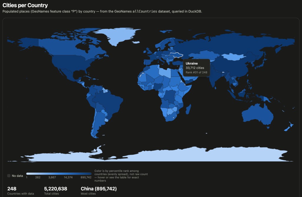
Aggregate analysis — total populated-place counts and summed population by country (China leads with 895,742 places), US timezone distribution (57 distinct IANA zones), and the 20 most recently modified records (GeoNames updates daily).
These are the kinds of queries that make real data worth the curation effort — and the kinds of questions you can ask an AI assistant to draft once the schema is in place.
A static snapshot, visualized with open source maps
This is a static dataset in two senses. First, the GeoNames source is a point-in-time export — the allCountries dump downloaded on a given date, not a live API. Second, the map visualization works from a fixed aggregation extracted from DuckDB and embedded directly in the HTML. The browser does not connect to DuckDB, R2, or any backend at runtime.
The workflow is deliberately simple:
- Query DuckDB locally — aggregate populated places (GeoNames feature class
P) by country code:
SELECT country_code, count(*) AS city_count
FROM geonames
WHERE feature_class = 'P'
GROUP BY country_code
ORDER BY 2 DESC;
- Export the result — a JSON object of country code → city count, baked into the page as
COUNTS - Render statically — no server, no database connection, no API keys at view time
That last point matters. Once built, the HTML file is fully self-contained. Open it from disk, email it, commit it to GitHub, or publish it as a Claude Code artifact — the visualization behaves the same everywhere.
Open source map stack
The map itself uses entirely open source, license-friendly components:
- Natural Earth — 110m country boundary polygons, embedded as GeoJSON in the page. Natural Earth data is public domain, widely used, and requires no tile server or mapping API subscription.
- SVG rendering — country shapes drawn as SVG paths in the browser, shaded by percentile rank using a blue colour ramp. Hover tooltips and a sortable data table are plain HTML and JavaScript.
- No Mapbox, no Google Maps, no proprietary tiles — the entire visualization runs from a single HTML file with zero external dependencies at runtime.
The GeoNames aggregation — 248 countries, 5,220,638 populated places, China leading with 895,742 cities — was produced by DuckDB. The map is just a portable rendering of that query result.
Publishing visualizations without hosting
One of the more interesting outcomes of this workflow is how AI changes the delivery of data, not just the preparation.
Working in Claude Code , I built the interactive world map shown in the hero image — populated places shaded by count per country, with hover tooltips, a percentile-ranked colour scale, and a sortable data table. The working session is preserved as a Claude Code artifact .
The key point: Claude Code artifacts publish directly. No web server, no S3 bucket, no deployment pipeline. You build the visualization in a session, and Claude hosts the result at a shareable URL. Anyone with the link can interact with it immediately.
For reproducibility, the same HTML is committed to the repository as city_density_map.html
. Download it and open it locally in any browser — the DuckDB-derived aggregation and Natural Earth country boundaries are embedded, so it runs entirely offline with no hosting requirements.
Free egress with Cloudflare R2
For programmatic access — querying the dataset from DuckDB without downloading 1.7 GB first — I took inspiration from the DuckDB Web Shell , which loads remote Parquet and CSV files directly into the browser.
The same pattern works from the DuckDB CLI using HTTP/S read functions. The GeoNames data is published on Cloudflare R2
at blobs.ronaldbradford.com, taking advantage of R2’s free egress — no per-GB download charges when querying from anywhere on the internet.
$ duckdb
D INSTALL httpfs; LOAD httpfs;
D SELECT count(*) FROM read_parquet('https://blobs.ronaldbradford.com/geonames/*.parquet');
┌──────────────┐
│ count_star() │
├──────────────┤
│   13455020   │
└──────────────┘
Point DuckDB at the remote Parquet files and query immediately — no local copy required. The same queries from geonames-queries.sql run unchanged against the remote data.
Compare this to the MySQL curation workflow from last week’s post, where each dataset needed a load script, index tuning, and often a multi-gigabyte local import before you could run a single query. DuckDB’s ability to query remote Parquet over HTTP, combined with R2’s free egress, changes the economics of publishing large reference datasets.
What AI changed — and what it did not
| Step | Before AI | With AI assistance |
|---|---|---|
| Schema design | Manual inspection of sample rows | Draft DDL from field documentation, iterate on type mismatches |
| Load scripts | Write and debug shell/SQL by hand | Generate COPY options, compression pipeline, index DDL |
| Query exploration | Write SQL from scratch | Describe intent in natural language, refine results |
| Visualization | Separate tooling, hosting setup | Extract aggregation from DuckDB; render with open source maps (Natural Earth + SVG); publish as static HTML |
| Data distribution | Local files or custom hosting | Parquet on R2 with free egress, queryable via DuckDB HTTP |
What did not change:
- Provenance — the data still comes from GeoNames under CC BY 4.0 . Attribution and licensing still matter.
- Validation — row counts, spot checks (Tingalpa at
-27.4736, 153.12704with population 8,051), and sanity queries on known places. - Reproducibility — scripts in the repository, not just a chat transcript. Anyone can rebuild from source.
The manual MySQL datasets in mysql-data/
remain valuable for engine-specific testing — replication, indexing behaviour, upgrade paths. The DuckDB datasets under free-download/
serve a different purpose: fast analytical exploration, interactive visualization, and remote querying without infrastructure.
More datasets are in progress. If you have a public data source worth curating, or want to collaborate on the R2-hosted collection, reach out via my Contact form .