Producing Two Sample T-Test statistics with SQL

The two sample t-test for equal variance is a statistical test to determine if the means of two groups are different enough that the difference is likely caused by some underlying difference, rather than random chance. The null hypothesis is that any difference in the means of the two groups is explainable by random chance.

In Chapter 2, of “Analytics Stories: Using Data to Make Good Things Happen” , the author Wayne L. Winston poses the question “Was the 1969 US Draft Lottery Fair?” A quote from the book.

Statisticians quickly noticed; see Statisticians Charge Draft Lottery Was Not Random ; that lottery numbers for the last few months of the year seemed to be suspiciously low, meaning that men with late-year birthdays were more likely to be drafted. Were the statisticians correct?

Using this example as part of coursework in the School of Business Masters Curriculum at Fairfield University I calculated t-test results with Excel, and then also with a Python Notebook. The source data is a simple table, available here .

Leveraging the VillageSQL Extension Bundle (VEB) , you can now calculate these statistics directly in SQL against the table, no additional product or calculation necessary. VillageSQL is a drop-in MySQL 8.4 replacement.

US Draft T-Test Example

T-Test SQL Example

-- Inference statistics for the 1969 draft (first-half vs second-half year)
SELECT CAST(STATS_TTEST(
    CAST(n69 AS DOUBLE),
    CASE
        WHEN month BETWEEN 1 AND 6  THEN 1
        WHEN month BETWEEN 7 AND 12 THEN 2
    END,
    0.05
) AS CHAR(1000)) AS ttest_1969
FROM us_draft
WHERE month BETWEEN 1 AND 12;

-- Per-group descriptives for the 1969 draft
SELECT CAST(STATS_TTEST_GROUPS(
    CAST(n69 AS DOUBLE),
    CASE
        WHEN month BETWEEN 1 AND 6  THEN 1
        WHEN month BETWEEN 7 AND 12 THEN 2
    END
) AS CHAR(1000)) AS ttest_groups_1969
FROM us_draft
WHERE month BETWEEN 1 AND 12;

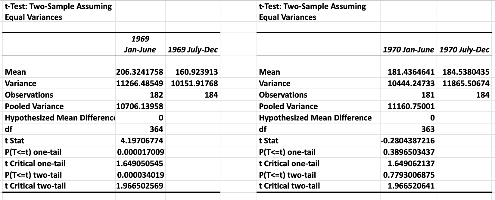
1969 Results

*************************** 1. row ***************************
          draft_year: 1969 Draft
        mean_jan_jun: 206.324175824176
        mean_jul_dec: 160.923913043478
    variance_jan_jun: 11266.4854896485
    variance_jul_dec: 10151.9176764077
observations_jan_jun: 182
observations_jul_dec: 184
     pooled_variance: 10706.1395835412
  degrees_of_freedom: 364
         t_statistic: 4.19706774041344
    p_value_one_tail: 0.000017009793217
 t_critical_one_tail: 1.64905054517173
    p_value_two_tail: 0.000034019586435
 t_critical_two_tail: 1.96650256879886
   hypothesis_result: Significant Difference

1970 Results

*************************** 2. row ***************************
          draft_year: 1970 Draft
        mean_jan_jun: 181.436464088398
        mean_jul_dec: 184.538043478261
    variance_jan_jun: 10444.2473296501
    variance_jul_dec: 11865.5067415063
observations_jan_jun: 181
observations_jul_dec: 184
     pooled_variance: 11160.7500083545
  degrees_of_freedom: 363
         t_statistic: -0.280438721554645
    p_value_one_tail: 0.3896503437259
 t_critical_one_tail: 1.64906213665239
    p_value_two_tail: 0.7793006874518
 t_critical_two_tail: 1.96652064056793
   hypothesis_result: No Significant Difference
2 rows in set (0.00 sec)

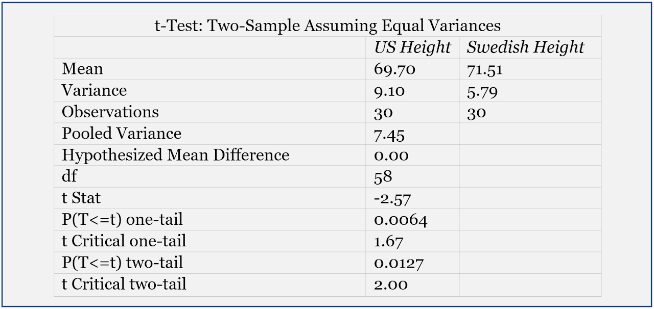
Comparing Population Heights

In this second SQL example I used the data found at Two Sample T-Test Equal Variance Comparing two Samples/Populations/Groups/Means/Values where you can find matching results.

 *************************** 1. row ***************************
            mean_us: 69.6960004170736
       mean_swedish: 71.5073333740234
        variance_us: 9.10271715155659
   variance_swedish: 5.79374292845484
               n_us: 30
          n_swedish: 30
    pooled_variance: 7.44823004000572
 degrees_of_freedom: 58
        t_statistic: -2.57049863701552
   p_value_one_tail: 0.00637231411898375
t_critical_one_tail: 1.67155276245484
   p_value_two_tail: 0.0127446282379675
t_critical_two_tail: 2.00171748414489
         conclusion: Reject Null — heights differ significantly